Cross-Category Calibration Analysis of Kalshi Mention Markets
Luiz Felipe Barbosa · 15 Mar 2026 · 10 min read
Prediction markets promise a very clean deal: the price is supposed to be the probability. If a contract trades at 70 cents, it should resolve YES about 70% of the time (Wolfers & Zitzewitz, 2006). When that relationship breaks, the interesting question is not just whether the market is wrong. It is how it is wrong, where it is wrong, and whether the error is random noise or something more structural.
Recent work by Bürgi, Deng, and Whelan (2025) shows that Kalshi exhibits a favorite–longshot bias at the exchange level. But aggregate results only get you so far. Mention markets are a much better laboratory for looking at calibration because they are repetitive, short-lived, and unusually legible: the same types of events recur, the contract wording is clean, and outcomes can be checked quickly. That makes them one of the best places to see whether the market is actually learning or just repeating the same pricing mistakes in slightly different costumes.
This article looks at 18,948 resolved mention contracts across 126 series in six categories: Politicians, Sports, Earnings, Entertainment, Finance, and Media/News. Using volume-weighted average prices (VWAPs) measured at multiple horizons before the last trade, I examine how well prices track realized outcomes, how quickly markets move toward fair probabilities, and whether the remaining errors survive Kalshi's fee schedule well enough to matter. The basic finding is simple. Mention markets do converge. They just do not all converge in the same way, or at the same speed.
The Dataset
The dataset is drawn from Kalshi, a CFTC-regulated prediction exchange. It combines trade-level records with contract metadata across 141 mention series.
In raw form, the sample contains 35,837 total markets. Of these, 33,587 have resolved. After filtering to contracts with recorded trades and valid VWAP computations, 18,948 contracts remain for analysis. The sample runs from January 2025 through March 2026 and includes roughly 7.6 million individual trades.
Each mention series is assigned to one of six categories based on its content domain:
- Trade data: individual trade records with timestamps, prices in cents (1–99), trade counts, and taker-side identification across 141 series.
- Market data: contract metadata including ticker, series, title, result, close time, volume, and open interest.
An additional 663 contracts from 28 series fall into an "Other" residual category. Politicians account for 39% of all analyzed contracts, and Sports adds another 28%. Together, those two categories make up about two-thirds of the full sample.
| Category | Series | Contracts | Description |
|---|---|---|---|
| Politicians | 32 | 7,320 | Trump rallies, White House press briefings, mayoral debates, congressional hearings |
| Sports | 13 | 5,383 | NFL, NBA, NCAA, MLB, UFC/MMA broadcasts |
| Earnings | 1 | 2,118 | Corporate earnings call mentions |
| Entertainment | 21 | 1,228 | Late night shows, award ceremonies, reality TV, podcasts |
| Media/News | 17 | 757 | Cable news programs such as Fox News, MSNBC, and CNN |
| Finance | 14 | 559 | Federal Reserve, ECB, SEC proceedings, and fintech CEO appearances |
The Settlement Lag Problem
A surprisingly important data issue in this project is the distinction between two timestamps attached to each contract: close_time, when Kalshi settles and pays out the market, and last_trade_time, the timestamp of the final recorded trade. Those are not interchangeable.
Settlement often lags the last trade by a wide margin. Across all mention markets:
- Median lag: 71 minutes (1.2 hours)
- 75th percentile: 202 minutes (3.4 hours)
- Maximum: 19,617 minutes (13.6 days)
- 53.2% of contracts have a settlement lag greater than 1 hour
- 22.6% exceed 4 hours
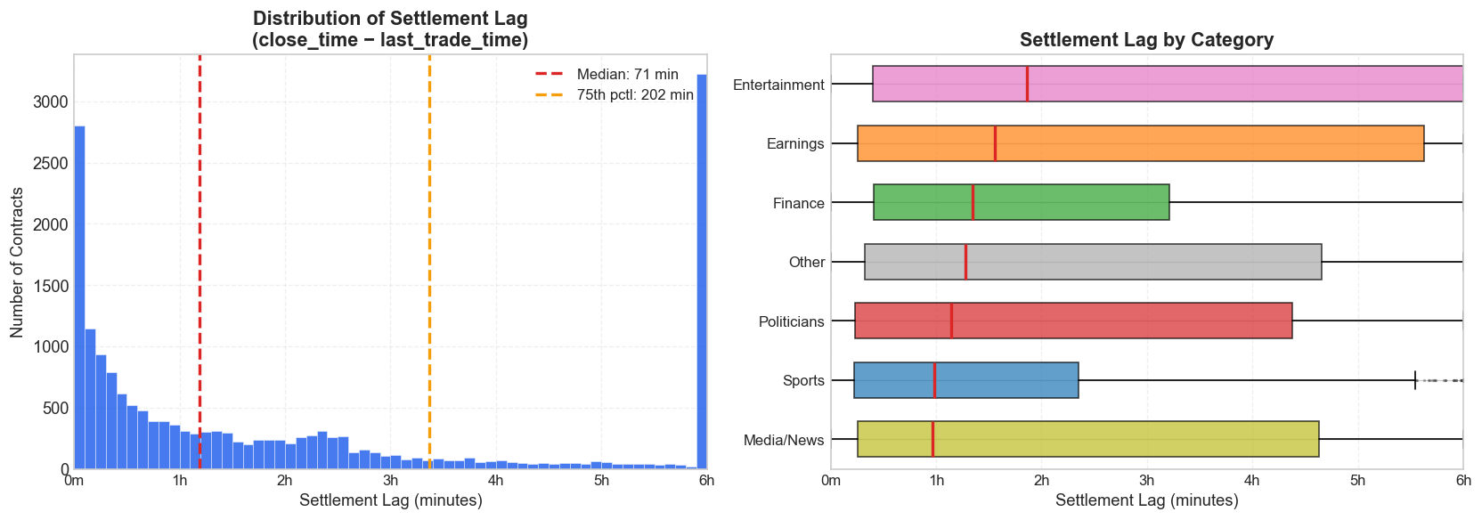
This matters because VWAP horizons need to be anchored to the moment trading actually stopped, not to the moment Kalshi eventually settled the contract. If a so-called 2-hour VWAP is anchored to settlement time, it may end up reflecting trades that occurred many hours before the market stopped moving. In extreme cases, the 10-minute, 30-minute, 1-hour, and 2-hour VWAPs all collapse to the same value simply because every trade happened before every cutoff.
In an earlier version of this analysis, I anchored VWAPs to close_time. That made roughly 82% of markets show vwap_2h equal to vwap_10m. After correcting the anchor to last_trade_time, that number falls to 17.7% — much closer to what one would expect from genuine early trading cessation rather than a timestamping artifact.
Methodology
For each resolved contract, I compute volume-weighted average prices at eight horizons before the last trade: 7 days, 3 days, 1 day, 6 hours, 2 hours, 1 hour, 30 minutes, and 10 minutes. The 2-hour VWAP serves as the main snapshot throughout the analysis because it balances recency with stability — close enough to capture late information, but not so close that a handful of final prints dominate the signal.
The VWAP at a given horizon is defined as:
where the cutoff is last_trade_time minus the relevant horizon. Prices are in cents, so a VWAP of 70 corresponds to a 70% market-implied YES probability.
Calibration is measured by sorting contracts into probability buckets based on VWAP and then comparing each bucket's implied probability to its realized YES rate. A perfectly calibrated market would sit on the 45-degree diagonal: contracts priced at 15% would resolve YES about 15% of the time.
To summarize calibration quality in a single number, I use Mean Absolute Deviation (MAD):
MAD is expressed in percentage points and is computed across all buckets with at least five observations. Lower values indicate better calibration.
Kalshi's taker fee schedule is also built directly into the backtests:
where p is the contract price in cents. Fees are highest near the middle of the probability range and decline toward the extremes, which matters because the largest calibration errors often show up precisely at those extremes.
To test whether miscalibration is economically meaningful rather than just statistically visible, I backtest two simple threshold strategies on the 2-hour VWAP:
- Buy YES: purchase YES contracts when the 2-hour VWAP exceeds a given threshold.
- Buy NO: purchase NO contracts when the 2-hour VWAP falls below a given threshold.
Thresholds are tested at 10-point intervals from 10% through 90%, and net PnL per trade is computed after deducting Kalshi taker fees.
Category-Level Calibration
The summary statistics reveal meaningful variation across categories:
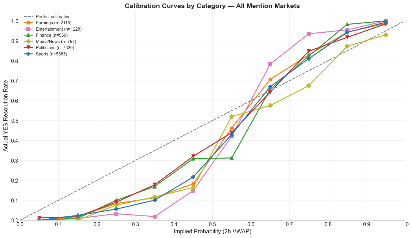
Directional accuracy — whether the 2-hour VWAP gets the direction right by predicting YES above 50 and NO below 50 — exceeds 83% in every category. Entertainment leads at 92.6%, but that partly reflects its low base rate: only 32.3% of entertainment contracts resolve YES, so a strategy that always predicts NO would already start with a structural advantage.
MAD tells a different story. Politicians have the lowest MAD at 9.5 percentage points, which suggests that the highest-volume category is also the best calibrated. Entertainment has the worst calibration at 16.4% despite the highest directional accuracy — exactly the kind of pattern one would expect when low-probability contracts are systematically mispriced rather than simply guessed in the wrong direction.
| Category | Contracts | YES Rate | Directional Accuracy | MAD (2h) |
|---|---|---|---|---|
| Earnings | 2,118 | 57.4% | 88.5% | 12.1% |
| Entertainment | 1,228 | 32.3% | 92.6% | 16.4% |
| Finance | 559 | 39.0% | 86.6% | 11.6% |
| Media/News | 757 | 40.8% | 83.6% | 11.2% |
| Politicians | 7,320 | 44.9% | 83.6% | 9.5% |
| Sports | 5,383 | 52.0% | 87.3% | 11.9% |
Multi-Horizon Calibration
Looking at a single snapshot misses the more interesting question: how does pricing improve as the event approaches? The next set of charts compares calibration curves across six horizons — from one day before the last trade down to ten minutes — for the four largest categories.
Earnings
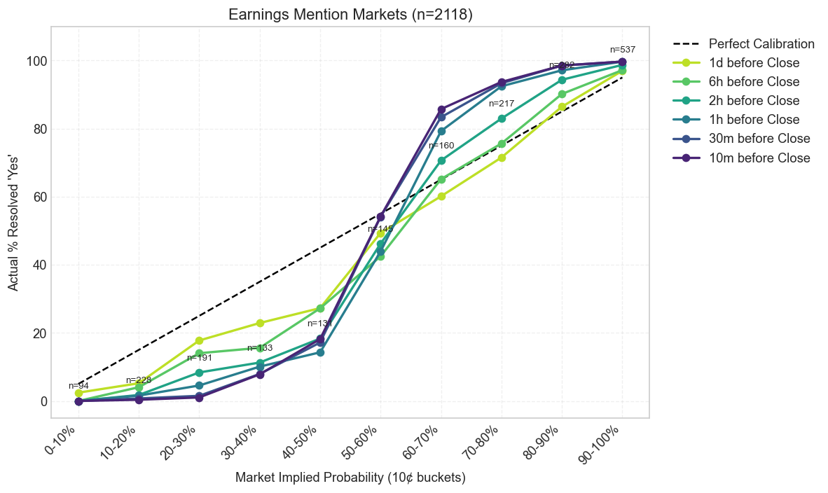
Every category improves as the event gets closer, which is what an informationally efficient market is supposed to do. But the speed of convergence is not the same across domains. Sports tightens early. Entertainment and Earnings stay noisy much longer. That difference matters because it suggests the market is not just learning over time; it is learning at different speeds depending on the structure of the underlying event.
Temporal Convergence
The same story becomes clearer when calibration is collapsed into MAD. All categories show improving calibration as the market approaches the final trade, and MAD declines monotonically from the 1-day horizon to the 10-minute horizon in every category. That is exactly what one would expect in an informationally efficient market as new information gets absorbed into price (Page & Clemen, 2013; Brown, Reade, & Vaughan Williams, 2019).
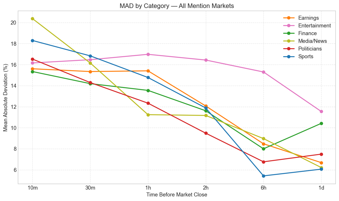
The rate of convergence, however, is not uniform. Some categories — especially Sports — reach fairly tight calibration by the 6-hour mark, while others, particularly Entertainment and Earnings, still retain meaningful error near the end. That suggests differences in information arrival: some events become legible early, while others remain genuinely unresolved until the final stretch. More broadly, it fits the larger prediction-market literature showing that calibration depends heavily on the information environment, the predictability of the event, and the depth of participation (Snowberg, Wolfers, & Zitzewitz, 2013).
Calibration Over Time
There is a second convergence question here. Even if prices improve within a contract's lifetime, has the market itself become better calibrated over the months of its existence? To answer that, I compute rolling cumulative MAD at weekly intervals for the four main categories.
Earnings
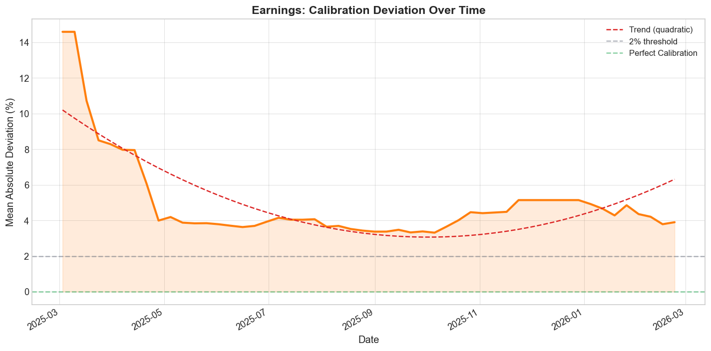
The category-level time series suggest that mention markets are learning. Calibration generally improves as more contracts are traded and resolved, though the slope is not identical across categories and some domains remain structurally noisier than others. That is one reason it makes more sense to think of mention markets as a family of related microstructures rather than as one homogeneous asset class.
Strategy Profitability
The backtest reveals a clear asymmetry between YES-side and NO-side strategies.
Buy YES becomes profitable above the 50% threshold and peaks at the 70% level, with average net PnL of +5.0 cents per trade across 6,424 trades. Returns taper at the 90% threshold because the hit rate rises but the remaining upside gets too small.
Buy NO is profitable across every tested threshold, with the strongest returns at the 40–50% range: +14.1 cents per trade at the <50% threshold across 8,152 trades. That reflects a persistent longshot bias — low-probability contracts resolve NO more often than their price implies, leaving the NO side systematically underpriced.
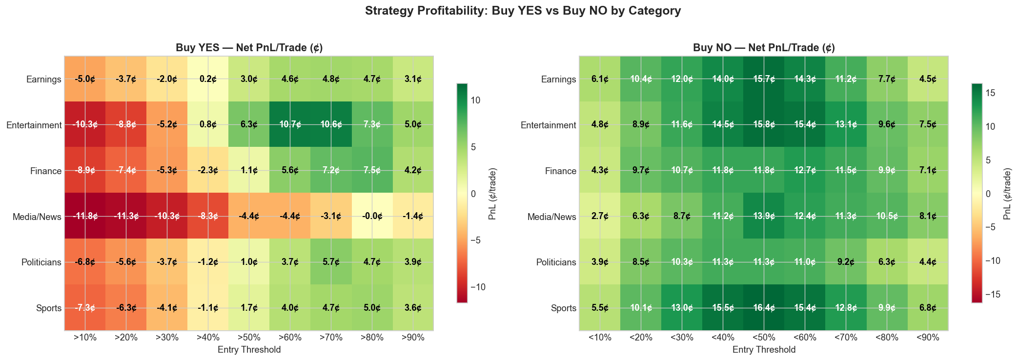
The asymmetry is not subtle. The best Buy NO threshold (<50%) averages +14.1 cents per trade, nearly three times the best Buy YES threshold. That implies the dominant miscalibration in mention markets sits on the low end of the probability distribution: traders systematically overestimate the chance that a word or phrase will be mentioned. The pattern lines up with the favorite–longshot bias documented in betting and prediction markets more broadly (Page & Clemen, 2013; Snowberg & Wolfers, 2010), including at the aggregate Kalshi level (Bürgi, Deng, & Whelan, 2025).
VWAP Price Trajectories
The spaghetti plots below show the VWAP trajectory for every contract in each main category, from seven days before the last trade down to ten minutes. Green traces resolve YES; red traces resolve NO. What they make visible is the broad separation between outcomes and the familiar funnel pattern as prices move toward 0 or 100 near resolution.
Earnings
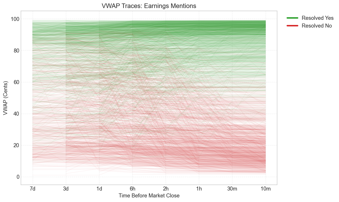
These plots are useful because they show the same phenomenon in less aggregated form. Calibration curves and heatmaps summarize the edge. The trajectories show how that edge actually develops over time. Some categories separate early and cleanly. Others stay tangled much longer, which is exactly what later shows up as higher residual MAD and weaker calibration.
Category-Specific Opportunities
Profitability is not uniform across categories. Entertainment and Earnings show especially large NO-side returns, which is consistent with their low YES rates and relatively poor calibration. Politicians, by contrast, are better calibrated overall but still produce attractive YES-side opportunities at high thresholds simply because the category is so large and liquid.
That distinction matters if the goal is actual deployment rather than just descriptive measurement. A category with the largest apparent mispricing is not automatically the most attractive one if liquidity is thin, fills are hard, or the edge is concentrated in only a small handful of contracts. What matters is the combination of mispricing, scale, and execution quality.
Limitations
There are a few obvious limits to how far these results should be pushed. The first is that the whole exercise is in-sample: I use the same data to describe the calibration errors and to evaluate the strategy rules built on top of them. That means the edge may look cleaner in hindsight than it would in live deployment, especially if these markets have already become more efficient over time.
The second is that the raw contract count overstates the amount of independent information in the sample. Many contracts are tied to the same underlying event — a single earnings call, sports broadcast, or political speech can generate a cluster of related mention markets that move together and often resolve together. So while the dataset is large, the effective sample size is smaller than the headline number suggests, and the backtests likely understate how lumpy real risk would feel.
The third is execution. The strategy results assume fills at the 2-hour VWAP, which is a useful benchmark but not a guaranteed tradeable price. They also leave out slippage, queue position, and the uneven fill dynamics of patient maker orders. Add in the fact that the sample excludes cancelled, delisted, and inactive contracts, and the safest way to read the backtests is as evidence of persistent mispricing — not as a turnkey estimate of what a live strategy would have earned dollar for dollar.
Conclusion
The cleanest way to put the result is this: mention markets are not broken, but they are not evenly efficient either. Prices do move toward fair probabilities as events approach. The problem is that some categories get there much faster than others, and the remaining mistakes are not randomly scattered across the probability range. The dominant error is still longshot bias. Low-probability mention contracts are too expensive, which means the NO side is systematically cheaper than it should be even after fees.
What matters most in the cross-category view is that the pattern is structural. Politicians — the largest category — is also the best calibrated, which is exactly what one would expect if repeated participation, stronger base rates, and deeper liquidity improve price quality. Smaller or structurally messier categories such as Entertainment and Finance drift further from fair value. In other words, the market is learning, but it is learning unevenly. Some formats get disciplined quickly. Others stay noisy for longer than they should.
That is probably the main takeaway. The interesting story here is not simply that Kalshi mention markets contain tradable errors. It is that the same contract design can produce very different calibration dynamics depending on the information environment around it. Whether that remaining gap amounts to durable alpha or just a temporary phase of market maturation is still an open question. But for now, there is enough error left in the system to be visible, interpretable, and in some categories, clearly worth paying attention to.
Works Cited
- Arrow, K.J., Forsythe, R., Gorham, M., Hahn, R., Hanson, R., et al. (2008). "The Promise of Prediction Markets." Science, 320(5878), 877–878. https://doi.org/10.1126/science.1157679
- Barbosa, L.F. (2026). mention-analysis [Computer software]. GitHub. https://github.com/LuizFelipeBarbosa/mention-analysis
- Brown, A., Reade, J.J., & Vaughan Williams, L. (2019). "When Are Prediction Market Prices Most Informative?" International Journal of Forecasting, 35(1), 420–428. https://doi.org/10.1016/j.ijforecast.2018.07.012
- Bürgi, C., Deng, W., & Whelan, K. (2025). "Makers and Takers: The Economics of the Kalshi Prediction Market." CEPR Discussion Paper No. 20631; CESifo Working Paper No. 12122. https://ssrn.com/abstract=5502658
- Kahneman, D. & Tversky, A. (1979). "Prospect Theory: An Analysis of Decision under Risk." Econometrica, 47(2), 263–291. https://doi.org/10.2307/1914185
- Kalshi. (2026). "Fee Schedule." https://kalshi.com/docs/kalshi-fee-schedule.pdf
- Kalshi Help Center. "How is Kalshi regulated?" https://help.kalshi.com/en/articles/13823765-how-is-kalshi-regulated
- Kalshi Help Center. "Limit Orders." https://help.kalshi.com/en/articles/13823811-limit-orders
- Page, L. & Clemen, R.T. (2013). "Do Prediction Markets Produce Well-Calibrated Probability Forecasts?" Economic Journal, 123(568), 491–513. https://doi.org/10.1111/j.1468-0297.2012.02561.x
- Snowberg, E. & Wolfers, J. (2010). "Explaining the Favorite–Long Shot Bias: Is It Risk-Love or Misperceptions?" Journal of Political Economy, 118(4), 723–746. https://doi.org/10.1086/655844
- Snowberg, E., Wolfers, J., & Zitzewitz, E. (2013). "Prediction Markets for Economic Forecasting." In Handbook of Economic Forecasting, Vol. 2, 657–687. Elsevier.
- Whelan, K. (2024). "Risk Aversion and Favourite–Longshot Bias in a Competitive Fixed-Odds Betting Market." Economica, 91(361), 188–209.
- Wolfers, J. & Zitzewitz, E. (2004). "Prediction Markets." Journal of Economic Perspectives, 18(2), 107–126. https://doi.org/10.1257/0895330041371321
- Wolfers, J. & Zitzewitz, E. (2006). "Interpreting Prediction Market Prices as Probabilities." NBER Working Paper No. 12200.
More Articles
An Analysis of PressTV and Three Privately-Owned Israeli News Channels on Telegram
12 May 2026A comparative NLP analysis of PressTV and three privately owned Israeli Telegram news channels, showing how ownership shapes cadence, topic structure, and media strategy while all four converge around a fear-dominant Iran-Israel-US frame.
Calibration Errors and Trading Opportunities in Kalshi Political Speech Mention Markets
27 Mar 2026A study of 7,320 Kalshi political speech mention contracts showing that these markets learn over time but still overprice low-probability YES outcomes, leaving the NO side materially stronger after fees.
Adorno’s Critique in the Age of the “For You” Page
25 Feb 2026This project analyzes 84,816 YouTube comments on the 15 most-streamed songs of 2025 to test Adorno’s Culture Industry. It finds that only 0.32% of comments critically engage with the production system behind pop music.